Linear regression - operace s maticemi
Užitečné odkazy
- Linear Regression
- Gradient Descent
- Machine Learning - Coursera.org
- Zdrojové kódy z cvičení formou notebooku
Motivace
V případě regression (oproti classification) má za úkol algoritmus predikovat ‘real-value’ hodnotu. Linear regression je jednoduchý přístup k supervised machine learning. Linear regression je používána na predikci hodnoty Y na základě hodnoty X, předpokládáme, že mezi těmito hodnotami je lineární závislost. I přes jeho jednoduchost je tento přístup ve světe machine learning stále používán.
In statistics, linear regression is a linear approach to modelling the relationship between a scalar response (or dependent variable) and one or more explanatory variables (or independent variables).
V ukázkách níže, jsou využity knihovny numpy a matplotlib. Knihovna numpy je nejrozšířenější knihovna pro matematické operace s vektory a maticemi, knihovna uvnitř spolupracuje s C++/Fortran kódem. Knihovna matplotlib pak slouží k vykreslování grafů.
1
2
3
4
5
6
7
8
9
10
11
12
13
14
15
16
17
18
19
import numpy as np
import matplotlib.pyplot as plt
import matplotlib
%matplotlib inline
def plot_regression_function(theta0, theta1):
line_x = np.linspace(3,25,100)
line_y = theta0 + theta1 * line_x
plt.plot(line_x, line_y, zorder=1, color='red')
def plot_data(X, Y, color='black'):
plt.scatter(X, Y, zorder=2, color=color, s=4)
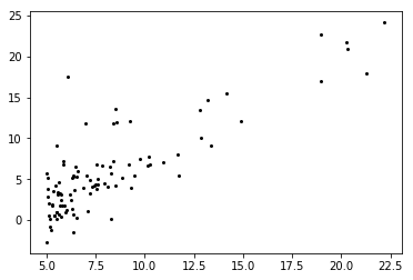
data = np.loadtxt('data.txt',delimiter=',')
# first column of dataset
X = data[:,0]
# second column of dataset
Y = data[:,1]
1
2
plot_data(X, Y)
plt.show()
1
2
3
4
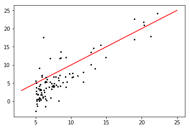
# plot y = 0 + 1 * x
plot_regression_function(0, 1)
plot_data(X, Y)
plt.show()
1
2
3
4
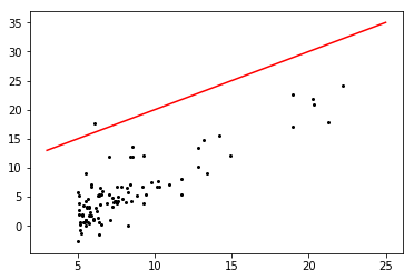
# plot y = 10 + 1 * x
plot_regression_function(10, 1)
plot_data(X, Y)
plt.show()
1
2
3
4
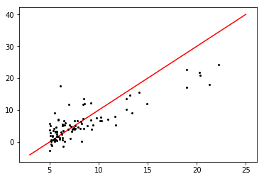
# plot y = -10 + 2 * x
plot_regression_function(-10, 2)
plot_data(X, Y)
plt.show()
Výpočet bez využítí matic a vektorizace
1
2
3
4
5
6
7
8
9
10
11
12
13
14
15
16
17
18
19
20
21
22
23
24
25
26
27
28
29
30
31
32
33
34
35
36
37
38
39
40
41
42
43
44
# linear model hypothesis
def hypothesis(X, theta0, theta1):
return theta0 + theta1 * X
def calculate_new_thetas(theta0, theta1, alpha):
sum_theta0 = 0
sum_theta1 = 0
for xi, yi in zip(X, Y):
sum_theta0 += hypothesis(xi, theta0, theta1) - yi
sum_theta1 += (hypothesis(xi, theta0, theta1) - yi) * xi
new_theta0 = theta0 - alpha * (1 / m) * sum_theta0
new_theta1 = theta1 - alpha * (1 / m) * sum_theta1
return new_theta0, new_theta1
# gradient descent alg for calculating thetas
def gradient_descent(theta0, theta1, max_iter, alpha):
for i in range(max_iter):
theta0, theta1 = calculate_new_thetas(theta0, theta1, alpha)
return theta0, theta1
theta0 = 0
theta1 = 0
alpha = 0.01
m = len(data)
X = data[:,0]
Y = data[:,1]
iterations = 1500
theta0, theta1 = gradient_descent(theta0, theta1, iterations, alpha)
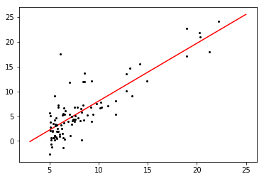
# --plotting--
plot_regression_function(theta0, theta1)
plot_data(X, Y)
plt.show()
# ------------
plt.show()

Výpočet s využítím matic a vektorizace
1
2
3
4
5
6
7
8
9
10
11
12
13
14
15
16
17
18
19
20
21
22
23
24
25
26
27
28
29
30
def hypothesis(X, theta):
    return np.transpose(theta).dot(X).flatten()

def gradient_descent(theta, max_iter):
    for i in range(max_iter):
        theta = np.subtract(
            theta, np.transpose(
                (np.multiply(
                    np.subtract(hypothesis(X, theta), Y), X) * (1 / m) * alpha).sum(axis=1).reshape([1, number_of_features])))

    return theta

number_of_features = 2
alpha = 0.01
m = len(data)

# add ones as first column of X, needed for calculation of hypothesis
X = np.vstack((np.ones(m), data[:,0]))
Y = data[:,1]

theta = np.zeros((number_of_features,1))
theta = gradient_descent(theta, 1500)

# --plotting--
plot_regression_function(theta[0][0], theta[1][0])
plot_data(X[1], Y)
plt.show()
# ------------

plt.show()
Predikce na základě získaných hodnot
1
2
3
4
5
6
7
8
9
10
11
12
13
14
15
16
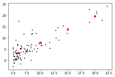
# plot training data
plot_data(X[1], Y)
# data for regression
regression = np.array([6, 10, 15, 20])
# add ones as first column of X, needed for calculation of hypothesis
regression_set_X = np.vstack((np.ones(len(predict)), predict))
# calculate values
regression_set_Y = hypothesis(regression_set_X, theta)
# plot results of regression
plt.scatter(precict_set_X[1], regression_set_Y, zorder=2, color='red')
plt.show()